Apply and compare several estimators to conduct a causal mediation analysis

Establish identifiability

med_bench implements several estimators for the natural direct and indirect causal effects. Before moving forward with estimation, the investigator should ensure that those causal effects are identified by discussing the plausability of the identification assumptions

• SUTVA (Stable Unit Treatment Values Assumption)

• Sequential ignorability of the treatment and the mediator(s), by selecting an adequate set of confounding variables that need to be adjusted on

• Positivity of the treatment and the mediator.

In this example we will admit those assumptions and simulate a dataset, with the following data generating process, with simple linear models.

\[X \sim \mathcal{N}(0, I_p)\]

\[T|X \sim \mbox{Bernoulli} (\mbox{expit}( a_0 + X^t a_X ))\]

\[M|X, T \sim b_0 + X^t b_X + b_T T + \mathcal{N}(0, \sigma_M^2)\]

\[Y|X, T, M \sim c_0 + c_T T+ X^t c_X + c_M M + \mathcal{N}(0, \sigma_Y^2)\]

We use the function simulate_data to obtain a full simulated dataset for mediation analysis.

from med_bench.get_simulated_data import simulate_data
from med_bench.estimation.mediation_coefficient_product import CoefficientProduct

from numpy.random import default_rng
import matplotlib.pyplot as plt
import seaborn as sns
import pandas as pd

rg = default_rng(42)

(x, t, m, y, total, theta_1, theta_0,
 delta_1, delta_0, p_t, th_p_t_mx) = \
    simulate_data(n=500,
                  rg=rg,
                  mis_spec_m=False,
                  mis_spec_y=False,
                  dim_x=5,
                  dim_m=1,
                  seed=5,
                  type_m='continuous',
                  sigma_y=0.5,
                  sigma_m=0.5,
                  beta_t_factor=0.2,
                  beta_m_factor=5)

We can check the true values of the effects

print_effects = ('total effect: {:.2f}\n'
                'direct effect: {:.2f}\n'
                'indirect effect: {:.2f}')
print('True effects')
print(print_effects.format(total, theta_1, delta_0))

True effects
total effect: 1.70
direct effect: 1.20
indirect effect: 0.50

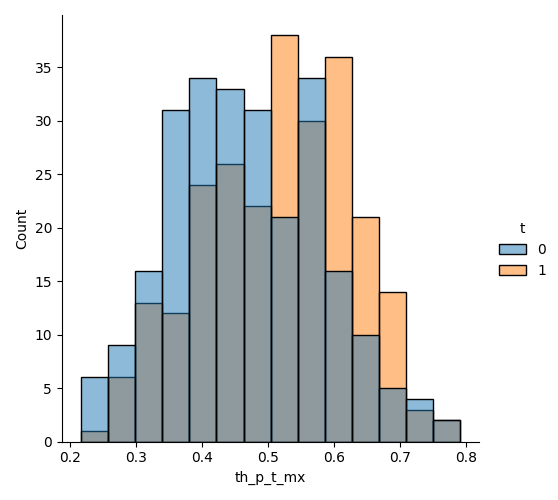
Contrary to the sequential ignorability assumption, the positivity assumption can be checked experimentally (not a guarantee but a good indication). We represent the distribution of \(P(T=1|X, M)\) for the treated and the untreated.

th_df = pd.DataFrame(zip(th_p_t_mx, t.ravel()), columns=['th_p_t_mx', 't'])
sns.displot(data=th_df, x='th_p_t_mx', hue='t')
plt.show()

Apply a baseline causal mediation estimator to your data: the coefficient product

We se that there are individuals from both treatment groups for all propensity values, which is supporting (bot not proving) the positivity assumption. Let’s now proceed with estimation. We begin with the simple coefficient product approach.

estimator = CoefficientProduct(regularize=False)
estimator.fit(t, m, x, y)
causal_effects = estimator.estimate(t.ravel(), m, x, y.ravel())
print('Estimated effects with the coefficient product')
print(print_effects.format(causal_effects["total_effect"],
                           causal_effects["direct_effect_treated"],
                           causal_effects["indirect_effect_control"]))

Nuisance models fitted
Estimated effects with the coefficient product
total effect: 1.78
direct effect: 1.23
indirect effect: 0.54

Comparaison with the other estimators

upcoming