Flexible use of an estimator in med_bench

In this example, we illustrate the different parameter choices when using an estimator. We can fit the model with different models for the estimation of nuisance parameters. It is also possible to use cross-fitting to compensate the estimation bias due to AI models.

We will also show bootstrap to obtain confidence intervals, and the different estimation variants regarding the choice of nuisance functions to estimate and the way to handle integration over the possible mediator values (not implemented yet in this example, stay tuned for more).

As in the previous example, we simulate data.

Data simulation

from med_bench.get_simulated_data import simulate_data
from med_bench.estimation.mediation_mr import MultiplyRobust

import numpy as np
from numpy.random import default_rng
import matplotlib.pyplot as plt
import seaborn as sns
import pandas as pd
from sklearn.ensemble import RandomForestClassifier, RandomForestRegressor
from sklearn.linear_model import LogisticRegressionCV, RidgeCV

ALPHAS = np.logspace(-5, 5, 8)
CV_FOLDS = 5
TINY = 1.0e-12

rg = default_rng(42)

(x, t, m, y, total, theta_1, theta_0,
 delta_1, delta_0, p_t, th_p_t_mx) = \
    simulate_data(n=500,
                  rg=rg,
                  mis_spec_m=False,
                  mis_spec_y=False,
                  dim_x=5,
                  dim_m=1,
                  seed=5,
                  type_m='continuous',
                  sigma_y=0.5,
                  sigma_m=0.5,
                  beta_t_factor=0.2,
                  beta_m_factor=5)
print_effects = ('total effect: {:.2f}\n'
                'direct effect: {:.2f}\n'
                'indirect effect: {:.2f}')
print('True effects')
print(print_effects.format(total, theta_1, delta_0))

res_list = list()

True effects
total effect: 1.70
direct effect: 1.20
indirect effect: 0.50

With simple linear models, without regularization

# define nuisance estimators with scikit-learn, without regularization
clf = LogisticRegressionCV(random_state=42, Cs=[np.inf], cv=CV_FOLDS)
reg = RidgeCV(alphas=[TINY], cv=CV_FOLDS)
estimator = MultiplyRobust(
    clip=1e-6, trim=0,
    prop_ratio="treatment",
    normalized=True,
    regressor=reg,
    classifier=clf,
    integration="implicit",
)
estimator.fit(t, m, x, y)
causal_effects_noreg = estimator.estimate(t.ravel(), m, x, y.ravel())
print(print_effects.format(causal_effects_noreg["total_effect"],
                           causal_effects_noreg["direct_effect_treated"],
                           causal_effects_noreg["indirect_effect_control"]))
res_list.append(['without regularization',
                 causal_effects_noreg["total_effect"],
                 causal_effects_noreg["direct_effect_treated"],
                 causal_effects_noreg["indirect_effect_control"]])

Nuisance models fitted
total effect: 1.78
direct effect: 1.23
indirect effect: 0.55

With simple linear models, with regularization

Regularization hyperparameters chosen by gridsearch and crossvalidation

clf = LogisticRegressionCV(random_state=42, Cs=ALPHAS, cv=CV_FOLDS)
reg = RidgeCV(alphas=ALPHAS, cv=CV_FOLDS)
estimator = MultiplyRobust(
    clip=1e-6, trim=0,
    prop_ratio="treatment",
    normalized=True,
    regressor=reg,
    classifier=clf,
    integration="implicit",
)
estimator.fit(t, m, x, y)
causal_effects_reg = estimator.estimate(t.ravel(), m, x, y.ravel())
print(print_effects.format(causal_effects_reg["total_effect"],
                           causal_effects_reg["direct_effect_treated"],
                           causal_effects_reg["indirect_effect_control"]))
res_list.append(['with regression',
                 causal_effects_reg["total_effect"],
                 causal_effects_reg["direct_effect_treated"],
                 causal_effects_reg["indirect_effect_control"]])

Nuisance models fitted
total effect: 1.78
direct effect: 1.25
indirect effect: 0.53

With machine learning models

clf = RandomForestClassifier(n_estimators=100,
                             min_samples_leaf=10,
                             max_depth=10,
                             random_state=25)
reg = RandomForestRegressor(n_estimators=100,
                            min_samples_leaf=10,
                            max_depth=10,
                            random_state=25)
estimator = MultiplyRobust(
    clip=1e-6, trim=0,
    prop_ratio="treatment",
    normalized=True,
    regressor=reg,
    classifier=clf,
    integration="implicit",
)
estimator.fit(t, m, x, y)
causal_effects_forest = estimator.estimate(t.ravel(), m, x, y.ravel())
print(print_effects.format(causal_effects_forest["total_effect"],
                           causal_effects_forest["direct_effect_treated"],
                           causal_effects_forest["indirect_effect_control"]))
res_list.append(['with RF',
                 causal_effects_forest["total_effect"],
                 causal_effects_forest["direct_effect_treated"],
                 causal_effects_forest["indirect_effect_control"]])

Nuisance models fitted
total effect: 1.82
direct effect: 1.27
indirect effect: 0.55

With cross-fitting

clf = RandomForestClassifier(n_estimators=100,
                             min_samples_leaf=10,
                             max_depth=10,
                             random_state=25)
reg = RandomForestRegressor(n_estimators=100,
                            min_samples_leaf=10,
                            max_depth=10,
                            random_state=25)
estimator = MultiplyRobust(
    clip=1e-6, trim=0,
    prop_ratio="treatment",
    normalized=True,
    regressor=reg,
    classifier=clf,
    integration="implicit",
)
cf_n_splits = 2
causal_effects_forest_cf = estimator.cross_fit_estimate(
    t, m, x, y, n_splits=cf_n_splits)
print(print_effects.format(causal_effects_forest_cf["total_effect"],
                           causal_effects_forest_cf["direct_effect_treated"],
                           causal_effects_forest_cf["indirect_effect_control"]))

res_list.append(['with RF CF',
                 causal_effects_forest_cf["total_effect"],
                 causal_effects_forest_cf["direct_effect_treated"],
                 causal_effects_forest_cf["indirect_effect_control"]])

Nuisance models fitted
Nuisance models fitted
total effect: 1.79
direct effect: 1.37
indirect effect: 0.42

Results summary

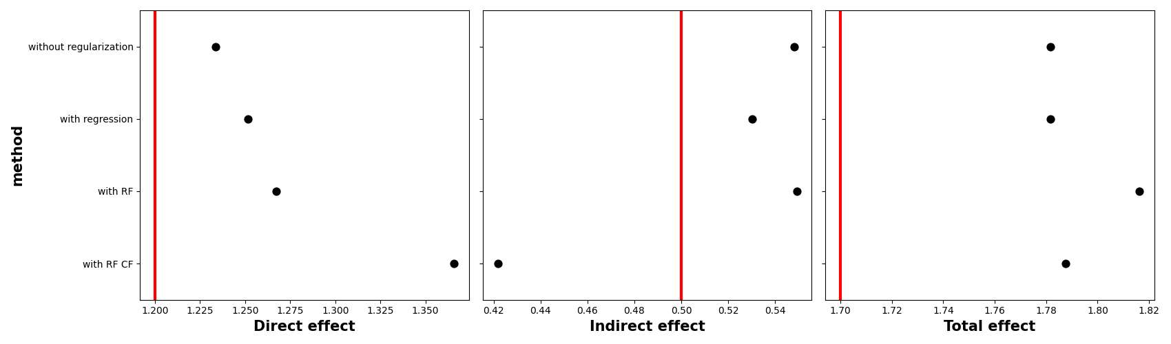
We show the estimates from the different methods, with the vertical red line being the theoretical value. In all cases we see a slight difference with the truth.

res_df = pd.DataFrame(res_list,
                      columns=['method',
                               'total_effect',
                               'direct_effect',
                               'indirect_effect'])
fig, ax = plt.subplots(ncols=3, figsize=(17, 5))
sns.pointplot(y='method', x='direct_effect', data=res_df, orient='h', ax=ax[0], join = False, color='black', estimator=np.median)

ax[0].set_ylabel('method', weight='bold', fontsize=15)
ax[0].set_xlabel('Direct effect', weight='bold', fontsize=15)
ax[0].axvline(x=theta_1, lw=3, color='red')
ax[1].axvline(x=delta_0, lw=3, color='red')
ax[2].axvline(x=total, lw=3, color='red')
sns.pointplot(y='method', x='indirect_effect', data=res_df, orient='h', ax=ax[1], join = False, color='black', estimator=np.median)
ax[1].set_ylabel('')
ax[1].set_xlabel('Indirect effect', weight='bold', fontsize=15)
ax[1].set(yticklabels=[])
sns.pointplot(y='method', x='total_effect', data=res_df, orient='h', ax=ax[2], join = False, color='black', estimator=np.median)
ax[2].set_ylabel('')
ax[2].set_xlabel('Total effect', weight='bold', fontsize=15)
ax[2].set(yticklabels=[])
plt.tight_layout()
plt.show()

/home/runner/work/med_bench/med_bench/docs/examples/example2.py:181: UserWarning:

The `join` parameter is deprecated and will be removed in v0.15.0. You can remove the line between points with `linestyle='none'`.

  sns.pointplot(y='method', x='direct_effect', data=res_df, orient='h', ax=ax[0], join = False, color='black', estimator=np.median)
/home/runner/work/med_bench/med_bench/docs/examples/example2.py:188: UserWarning:

The `join` parameter is deprecated and will be removed in v0.15.0. You can remove the line between points with `linestyle='none'`.

  sns.pointplot(y='method', x='indirect_effect', data=res_df, orient='h', ax=ax[1], join = False, color='black', estimator=np.median)
/home/runner/work/med_bench/med_bench/docs/examples/example2.py:192: UserWarning:

The `join` parameter is deprecated and will be removed in v0.15.0. You can remove the line between points with `linestyle='none'`.

  sns.pointplot(y='method', x='total_effect', data=res_df, orient='h', ax=ax[2], join = False, color='black', estimator=np.median)